Linear Regression in Python
In this post I wanted to show how to write from scratch a linear regression class in Python and then how to use it to make predictions. Let’s start!
What is Linear Regression
Linear regression is a technique of modelling a linear relationship between a dependent variable and independent variables. When the independent variable is just one, it is known as Simple Linear Regression, otherwise it is known as Multiple Linear Regression. The class we will build will deal with both. Linear Regression makes certain assumptions, such as the lack of multicollinearity which happens when two or more predictor variables are perfectly correlated.
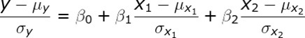
Given a vector of dependent variables y (M x 1) and a matrix of independent (predictor) variables X (M x N), linear regression assumes that their relationship is linear and can be written as:
![]()
Our goal will be to find the values of B that minimize the sum of squared errors:
where an error is defined as the difference between the predicted value: b0 + b1X1 + b2X2 and the observed value Y.
In order to do that, we will use a technique called Gradient Descent.
Gradient Descent
Gradient descent is an iterative algorithm which finds the minimum of a function. In our case, the function we are trying to minimize is the Cost function shown above. To make it easy to understand, imagine we’re dealing with a Simple Linear Regression scenario. This means that relationship is defined by:
![]()
And the Cost function to minimize is:
In order to find the minimum, we first need to compute the derivative of the cost function with respect to B0, which is:
![]()
then we start by assigning a random value to B0, we calculate the derivative and we decrease or increase the value of B0 by the calculated derivative. If the derivative is positive, it means the slope is positive therefore we need to decrease the value of B0, and need to do the contrary if the value of the derivative is negative. The new value is:
where alpha is a learning rate. We need to repeat this process iteratively until the value of the derivative is zero (function has reached its minimum).
But, as you have seen above, we also need to estimate the value of B1, therefore we also need to calculate the derivative with respect to B1 and repeat the same process. The vector containing the partial derivatives of a function with respect to different parameters is known as gradient. And so our gradient is:
Our class will then need to calculate the derivative of the cost function with respect to each coefficient, then calculate the new coefficients and repeat this process until the minimum has been reached.
Standard score
1 2 | def __init__(self, standardize=False): self._standardize = standardize |
1 2 3 4 5 6 7 8 9 10 11 12 13 14 15 16 17 18 19 20 21 22 23 | def predict(self, predictors: np.ndarray, coefficients: np.ndarray): ''' PARAMETERS ------------------- predictors: a N x M matrix where N is the number of observations and M is the number of attributes. The values in the first column are all 1's which are multiplied against the intercept coefficients: a M x 1 matrix where M is the number of attributes of predictors. DESCRIPTION ---------------------- Dot product of each row of predictors with coefficients equivalent to a matrix multiplication (N x M) * (M x 1) = (N x 1) RETURNS ---------------------- a N x 1 matrix where each element is a dot product of each observation with the respective coefficient ''' return np.matmul(predictors, coefficients) |
_errors method:
The _errors method is used to output a vector of the differences between the observed values (ys) and the predicted values:
1 2 3 4 5 6 7 8 9 10 11 12 13 14 15 16 17 18 19 20 | def _errors(self, ys: np.ndarray, coefficients: np.ndarray, predictors: np.ndarray): ''' PARAMETERS ------------------- predictors: a N x M matrix where N is the number of observations and M is the number of attributes. The values in the first column are all 1's which are multiplied against the intercept coefficients: a M x 1 matrix where M is the number of attributes of predictors. ys: a N x 1 matrix of the dependent variables where N is the number of observations RETURNS -------------------- N x 1 matrix of each observation error ''' predictions = self.predict(predictors, coefficients) return ys - predictions |
_sum_of_errors method:
The _sum_of_errors method returns the sum of the vector of _errors:
1 2 3 4 5 6 7 8 9 10 11 12 13 14 15 16 17 18 19 | def _sum_of_errors(self, ys: np.ndarray, coefficients: np.ndarray, predictors: np.ndarray): ''' PARAMETERS ------------------- predictors: a N x M matrix where N is the number of observations and M is the number of attributes. The values in the first column are all 1's which are multiplied against the intercept coefficients: a M x 1 matrix where M is the number of attributes of predictors. ys: a N x 1 matrix of the dependent variables where N is the number of observations RETURNS -------------------- the sum of the errors ''' return np.sum(self._errors(ys, coefficients, predictors)) |
_sum_of_squared_errors method:
The _sum_of_errors method returns the sum of the squared elements of _errors:
1 2 3 4 5 6 7 8 9 10 11 12 13 14 15 16 17 18 19 | def sum_of_squared_errors(self, ys: np.ndarray, coefficients: np.ndarray, predictors: np.ndarray): ''' PARAMETERS ------------------- predictors: a N x M matrix where N is the number of observations and M is the number of attributes. The values in the first column are all 1's which are multiplied against the intercept coefficients: a M x 1 matrix where M is the number of attributes of predictors. ys: a N x 1 matrix of the dependent variables where N is the number of observations RETURNS -------------------- the sum of squared errors ''' return np.sum(self._errors(ys, coefficients, predictors)**2) |
_derivatives method:
The _derivatives method will return a vector of the derivatives corresponding to the jth attribute:
1 2 3 4 5 6 7 8 9 10 11 12 13 14 15 16 17 18 19 20 21 22 23 24 25 26 27 | def _derivatives(self, ys: np.ndarray, coefficients: np.ndarray, predictors: np.ndarray, jth_column: int): ''' PARAMETERS ------------ ys: a N x 1 matrix of the dependent variables where N is the number of observations coefficients: a M x 1 matrix where M is the number of attributes of predictors. predictors: a N x M matrix where N is the number of observations and M is the number of attributes. The values in the first column are all 1's which are multiplied against the intercept jth_column: the index of the jth column of predictors RETURNS ---------- a N x 1 matrix of the partial derivatives with respect to the jth coefficient ''' # calculate the errors errors = self._errors(ys, coefficients, predictors) # extract jth column from predictors, reshape to N x 1 predictors_column = predictors[::, jth_column].reshape(-1, 1) # calculate the derivatives with respect to jth column: return -predictors_column * errors |
_new_coefficients method:
This method will return a vector of new coefficients calculated:
1 2 3 4 5 6 7 8 9 10 11 12 13 14 15 16 17 18 19 20 21 22 23 24 25 26 27 28 29 | def _new_coefficients(self, ys: np.ndarray, coefficients: np.ndarray, predictors: np.ndarray, learning_rate: float): ''' PARAMETERS ------------ ys: a N x 1 matrix of the dependent variables where N is the number of observations coefficients: a M x 1 matrix where M is the number of attributes of predictors. predictors: a N x M matrix where N is the number of observations and M is the number of attributes. The values in the first column are all 1's which are multiplied against the intercept learning_rate: the learning rate RETURNS ---------- a N x 1 matrix of the new calculate coefficients ''' new_coefficients = [] # iterate through the coefficients for index, coefficient in enumerate(coefficients, 0): # calculate all the derivatives with respect to the cofficient at position Index derivatives = self._derivatives(ys, coefficients, predictors, index) # calculate new coefficient new_coeffient = coefficient[0] - learning_rate * np.mean(derivatives) new_coefficients.append([new_coeffient]) return np.array(new_coefficients) |
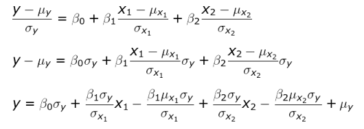
standardization methods:
The below methods are used to standardize and de-standardize the observed values (ys), the predictors variables(xs) and the coefficients:
1 2 3 4 5 6 7 8 9 10 11 12 13 14 15 16 17 18 19 20 21 22 23 24 25 26 27 28 29 30 31 32 33 34 35 36 37 38 39 40 41 42 43 44 45 46 47 48 49 50 51 52 53 54 55 56 57 58 59 60 61 | def _standardize_matrix(self, matrix:np.ndarray, mus:float, sigmas:float): ''' DESCRIPTION ------------ Standardize a matrix: (X - mu) / sigma PARAMETERS ----------- matrix: A np.ndarray of size N x M mus: a 1 x M np.ndarray containing the means sigmas: a 1 x M np.ndarray containing the standard deviations RETURNS ----------- The modified matrix ''' return (matrix - mus) / sigmas def _destandardize_matrix(self, matrix:np.ndarray, mu:float, sigma: float): ''' DESCRIPTION ------------ de-standardize a matrix: X * sigma + mu PARAMETERS ----------- matrix: A np.ndarray of size N x M mus: a 1 x M np.ndarray containing the original means sigmas: a 1 x M np.ndarray containing the original standard deviations RETURNS ----------- The modified matrix ''' return matrix * sigma + mu def _standardize_predictors(self, predictors:np.ndarray): ''' standardizes the predictors, stores the original means and standard deviations ''' self._predictors_mus = predictors.mean(axis=0) self._predictors_sigmas = predictors.std(axis=0) return self._standardize_matrix(predictors, self._predictors_mus, self._predictors_sigmas) def _standardize_ys(self, ys:np.ndarray): ''' standardizes the ys and stores the original means and standard deviations ''' self._ys_mus = ys.mean(axis=0) self._ys_sigmas = ys.std(axis=0) return self._standardize_matrix(ys, self._ys_mus, self._ys_sigmas) def _destandardize_thetas(self): # de standardize the intercept self.thetas[0] = self.thetas[0] * self._ys_sigmas + self._ys_mus - \ np.sum((self.thetas[1:] * self._predictors_mus.reshape(-1,1) * self._ys_sigmas) / self._predictors_sigmas.reshape(-1,1)) # de standardize the coefficients self.thetas[1:] = (self.thetas[1:] * self._ys_sigmas) / self._predictors_sigmas.reshape(-1,1) |
fit method:
The fit method is the one used to find the best values for the coefficients:
1 2 3 4 5 6 7 8 9 10 11 12 13 14 15 16 17 18 19 20 21 22 23 24 25 26 27 28 29 30 31 32 33 34 35 36 37 38 39 40 41 42 43 44 45 46 47 48 49 50 51 52 53 54 55 56 57 58 59 60 | def fit(self, predictors: np.ndarray, ys: np.ndarray, learning_rate=0.1, max_iters=10000): ''' DESCRIPTION ----------- finds the coefficients of a linear regression PARAMETERS ---------- predictors: a N x M array whose first column is a column 1's ys: a N x 1 matrix of the observed values learning_rate: the learning rate applied to the gradient descent algorithm, try smaller values if function does not converge max_iters: the maximum number of iterations used to find the coefficients ''' # store xs shape xs_rows, xs_columns = predictors.shape # add column of 1's to predictors self._predictors = predictors self._ys = ys # start with random coefficients self.thetas = np.random.randn(xs_columns, 1) # standardize predictors (except for 1st column) and ys self._predictors[::, 1:] = self._standardize_predictors(self._predictors[::, 1:]) self._ys = self._standardize_ys(self._ys) # get value of cost function # ((b0 + b1 * X1 + .... + bn * Xn) - y) / (2N) squared_errors = self.sum_of_squared_errors(self._ys, self.thetas, self._predictors) / (2 * xs_rows) for i in range(max_iters): # calculate new coefficients self.thetas = self._new_coefficients(self._ys, self.thetas, self._predictors, learning_rate) # new value of cost function new_squared_errors = self.sum_of_squared_errors(self._ys, self.thetas, self._predictors) / (2 * xs_rows) # if precision reached, return coefficients if new_squared_errors == squared_errors: break squared_errors = new_squared_errors # de standardize thetas if normalize is set to False if self._standardize == False: self._destandardize_thetas() self._ys = self._destandardize_matrix(self._ys, self._ys_mus, self._ys_sigmas) self._predictors[::, 1:] = self._destandardize_matrix(self._predictors[::, 1:], self._predictors_mus, self._predictors_sigmas) |
Other properties:
Below are three more properties available within the class:
- Intercept: returns the intercept (b0)
- coefficients: returns the coefficients (b1,…,bm)
- R_squared returns the coefficient of determination
1 2 3 4 5 6 7 8 9 10 | @property def intercept(self): return self.thetas[0] @property def coefficients(self): return self.thetas[1:] def R_squared(self, ys:np.ndarray, predictors:np.ndarray): return 1 - self.sum_of_squared_errors(ys, self.thetas, predictors) / np.sum((ys - np.mean(ys, axis=0)) ** 2) |
Below you will find the full class code:
1 2 3 4 5 6 7 8 9 10 11 12 13 14 15 16 17 18 19 20 21 22 23 24 25 26 27 28 29 30 31 32 33 34 35 36 37 38 39 40 41 42 43 44 45 46 47 48 49 50 51 52 53 54 55 56 57 58 59 60 61 62 63 64 65 66 67 68 69 70 71 72 73 74 75 76 77 78 79 80 81 82 83 84 85 86 87 88 89 90 91 92 93 94 95 96 97 98 99 100 101 102 103 104 105 106 107 108 109 110 111 112 113 114 115 116 117 118 119 120 121 122 123 124 125 126 127 128 129 130 131 132 133 134 135 136 137 138 139 140 141 142 143 144 145 146 147 148 149 150 151 152 153 154 155 156 157 158 159 160 161 162 163 164 165 166 167 168 169 170 171 172 173 174 175 176 177 178 179 180 181 182 183 184 185 186 187 188 189 190 191 192 193 194 195 196 197 198 199 200 201 202 203 204 205 206 207 208 209 210 211 212 213 214 215 216 217 218 219 220 221 222 223 224 225 226 227 228 229 230 231 232 233 234 235 236 237 238 239 240 241 242 243 244 245 246 247 248 249 250 251 252 253 254 255 256 257 258 259 260 261 262 263 264 265 266 267 268 269 270 271 272 273 274 275 276 277 278 279 280 281 282 283 284 285 286 287 288 289 290 291 292 293 294 295 296 297 298 299 300 301 302 303 | import numpy as np #import pandas as pd class LinearRegression(object): ''' DESCRIPTION -------------- Ordinary least squares Linear Regression class. Uses gradient descend algorithm to find the best thetas. The predictors are standardized before starting to find the best thetas (X - mu) / sigma If standardize is set to False then the thetas are de-standardized after the algorithm is done When using the 'predict' method, the matrix passed must contain 1's as the first column ''' def __init__(self, standardize=False): self._standardize = standardize def predict(self, predictors: np.ndarray, coefficients: np.ndarray): ''' PARAMETERS ------------------- predictors: a N x M matrix where N is the number of observations and M is the number of attributes. The values in the first column are all 1's which are multiplied against the intercept coefficients: a M x 1 matrix where M is the number of attributes of predictors. DESCRIPTION ---------------------- Dot product of each row of predictors with coefficients equivalent to a matrix multiplication (N x M) * (M x 1) = (N x 1) RETURNS ---------------------- a N x 1 matrix where each element is a dot product of each observation with the respective coefficient ''' # return np.sum(coefficients * predictors, axis=1) return np.matmul(predictors, coefficients) def sum_of_squared_errors(self, ys: np.ndarray, coefficients: np.ndarray, predictors: np.ndarray): ''' PARAMETERS ------------------- predictors: a N x M matrix where N is the number of observations and M is the number of attributes. The values in the first column are all 1's which are multiplied against the intercept coefficients: a M x 1 matrix where M is the number of attributes of predictors. ys: a N x 1 matrix of the dependent variables where N is the number of observations RETURNS -------------------- the sum of squared errors ''' return np.sum(self._errors(ys, coefficients, predictors)**2) def _sum_of_errors(self, ys: np.ndarray, coefficients: np.ndarray, predictors: np.ndarray): ''' PARAMETERS ------------------- predictors: a N x M matrix where N is the number of observations and M is the number of attributes. The values in the first column are all 1's which are multiplied against the intercept coefficients: a M x 1 matrix where M is the number of attributes of predictors. ys: a N x 1 matrix of the dependent variables where N is the number of observations RETURNS -------------------- the sum of the errors ''' return np.sum(self._errors(ys, coefficients, predictors)) def _errors(self, ys: np.ndarray, coefficients: np.ndarray, predictors: np.ndarray): ''' PARAMETERS ------------------- predictors: a N x M matrix where N is the number of observations and M is the number of attributes. The values in the first column are all 1's which are multiplied against the intercept coefficients: a M x 1 matrix where M is the number of attributes of predictors. ys: a N x 1 matrix of the dependent variables where N is the number of observations RETURNS -------------------- N x 1 matrix of each observation error ''' predictions = self.predict(predictors, coefficients) return ys - predictions def _derivatives(self, ys: np.ndarray, coefficients: np.ndarray, predictors: np.ndarray, jth_column: int): ''' PARAMETERS ------------ ys: a N x 1 matrix of the dependent variables where N is the number of observations coefficients: a M x 1 matrix where M is the number of attributes of predictors. predictors: a N x M matrix where N is the number of observations and M is the number of attributes. The values in the first column are all 1's which are multiplied against the intercept jth_column: the index of the jth column of predictors RETURNS ---------- a N x 1 matrix of the partial derivatives with respect to the jth coefficient ''' # calculate the errors errors = self._errors(ys, coefficients, predictors) # extract jth column from predictors, reshape to N x 1 predictors_column = predictors[::, jth_column].reshape(-1, 1) # calculate the derivatives with respect to jth column: # 2 * -xj * (y - (b0*1 + b1*x1 + .... + bn*xn)) #return 2 * -predictors_column * errors return -predictors_column * errors def _new_coefficients(self, ys: np.ndarray, coefficients: np.ndarray, predictors: np.ndarray, learning_rate: float): ''' PARAMETERS ------------ ys: a N x 1 matrix of the dependent variables where N is the number of observations coefficients: a M x 1 matrix where M is the number of attributes of predictors. predictors: a N x M matrix where N is the number of observations and M is the number of attributes. The values in the first column are all 1's which are multiplied against the intercept learning_rate: the learning rate RETURNS ---------- a N x 1 matrix of the new calculate coefficients ''' new_coefficients = [] # iterate through the coefficients for index, coefficient in enumerate(coefficients, 0): # calculate all the derivatives with respect to the cofficient at position Index derivatives = self._derivatives(ys, coefficients, predictors, index) # calculate new coefficient new_coeffient = coefficient[0] - learning_rate * np.mean(derivatives) new_coefficients.append([new_coeffient]) return np.array(new_coefficients) def _standardize_matrix(self, matrix:np.ndarray, mus:float, sigmas:float): ''' DESCRIPTION ------------ Standardize a matrix: (X - mu) / sigma PARAMETERS ----------- matrix: A np.ndarray of size N x M mus: a 1 x M np.ndarray containing the means sigmas: a 1 x M np.ndarray containing the standard deviations RETURNS ----------- The modified matrix ''' return (matrix - mus) / sigmas def _destandardize_matrix(self, matrix:np.ndarray, mu:float, sigma: float): ''' DESCRIPTION ------------ de-standardize a matrix: X * sigma + mu PARAMETERS ----------- matrix: A np.ndarray of size N x M mus: a 1 x M np.ndarray containing the original means sigmas: a 1 x M np.ndarray containing the original standard deviations RETURNS ----------- The modified matrix ''' return matrix * sigma + mu def _standardize_predictors(self, predictors:np.ndarray): ''' standardizes the predictors, stores the original means and standard deviations ''' self._predictors_mus = predictors.mean(axis=0) self._predictors_sigmas = predictors.std(axis=0) return self._standardize_matrix(predictors, self._predictors_mus, self._predictors_sigmas) def _standardize_ys(self, ys:np.ndarray): ''' standardizes the ys and stores the original means and standard deviations ''' self._ys_mus = ys.mean(axis=0) self._ys_sigmas = ys.std(axis=0) return self._standardize_matrix(ys, self._ys_mus, self._ys_sigmas) def _destandardize_thetas(self): # de standardize the intercept self.thetas[0] = self.thetas[0] * self._ys_sigmas + self._ys_mus - \ np.sum((self.thetas[1:] * self._predictors_mus.reshape(-1,1) * self._ys_sigmas) / self._predictors_sigmas.reshape(-1,1)) # de standardize the coefficients self.thetas[1:] = (self.thetas[1:] * self._ys_sigmas) / self._predictors_sigmas.reshape(-1,1) @property def intercept(self): return self.thetas[0] @property def coefficients(self): return self.thetas[1:] def R_squared(self, ys:np.ndarray, predictors:np.ndarray): return 1 - self.sum_of_squared_errors(ys, self.thetas, predictors) / np.sum((ys - np.mean(ys, axis=0)) ** 2) def fit(self, predictors: np.ndarray, ys: np.ndarray, learning_rate=0.1, max_iters=10000): ''' DESCRIPTION ----------- finds the coefficients of a linear regression PARAMETERS ---------- predictors: a N x M array whose first column is a column 1's ys: a N x 1 matrix of the observed values learning_rate: the learning rate applied to the gradient descent algorithm, try smaller values if function does not converge max_iters: the maximum number of iterations used to find the coefficients ''' # store xs shape xs_rows, xs_columns = predictors.shape # add column of 1's to predictors self._predictors = predictors self._ys = ys # start with random coefficients self.thetas = np.random.randn(xs_columns, 1) # standardize predictors (except for 1st column) and ys self._predictors[::, 1:] = self._standardize_predictors(self._predictors[::, 1:]) self._ys = self._standardize_ys(self._ys) # get value of cost function # ((b0 + b1 * X1 + .... + bn * Xn) - y) / (2N) squared_errors = self.sum_of_squared_errors(self._ys, self.thetas, self._predictors) / (2 * xs_rows) for i in range(max_iters): # calculate new coefficients self.thetas = self._new_coefficients(self._ys, self.thetas, self._predictors, learning_rate) # new value of cost function new_squared_errors = self.sum_of_squared_errors(self._ys, self.thetas, self._predictors) / (2 * xs_rows) # if precision reached, return coefficients if new_squared_errors == squared_errors: break squared_errors = new_squared_errors # de standardize thetas if normalize is set to False if self._standardize == False: self._destandardize_thetas() self._ys = self._destandardize_matrix(self._ys, self._ys_mus, self._ys_sigmas) self._predictors[::, 1:] = self._destandardize_matrix(self._predictors[::, 1:], self._predictors_mus, self._predictors_sigmas) |
Normal Equation
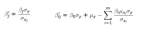
Normal equation is an alternative to gradient descend to find the coefficients which minimize the cost function. We need to think about this in terms of matrix calculus where the cost function becomes:
where X is a (m X n) matrix, theta is a (n X 1) matrix and Y is a (m x 1) matrix. If we calculate the derivative and solve for theta we get a vector of coefficients which minimize this cost function:
![]()
In this case, the fit method of my previous post, which is used to find the coefficients that minimize the cost function, becomes much simpler:
1 2 3 | def fit(self, X, Y): transposed_x = np.transpose(X) self.thetas = np.matmul(np.matmul(np.linalg.inv(np.matmul(transposed_x, X)), transposed_x), Y) |
It is worth nothing that this method will only work if the below matrix is invertible
![]()
Using the class we have created
Simple Linear Regression
The data set we will use for simple linear regression can be downloaded at this link. It is a simple data set containing two column with car insurance data. Column 1 contains our predictor variables (number of claims for a specific region) and column 2 contains our Ys (total payment for all the claims in thousands)
1 2 3 4 5 6 7 8 9 10 11 12 13 14 15 16 17 18 19 20 21 | from LinearRegression import LinearRegression import pandas as pd import numpy as np # load the data data = pd.read_csv(r'datasets\auto_insurance.csv') # get ys ys = data[['total_payments']].to_numpy() # get predictors and add 1 column with 1's xs = data[['number_of_claims']].to_numpy() xs = np.hstack((np.ones((xs.shape[0],1)), xs)) # calculate the coefficients L = LinearRegression() L.fit(xs, ys) print('Intercept is {0}'.format(L.intercept)) print('Coefficients are: {0}'.format(L.coefficients)) print('R^2 is: {0:4f}'.format(L.R_squared(ys, xs))) |
or in a Jupyter notebook:
Files can also be downloaded here: https://github.com/LivioLanzo/LinearRegressionPython