Logistic Regression
Logistic regression is a technique which can be applied to traditional statistics as well as machine learning. It is used to predict whether something is true or false and can be used to model binary dependent variables, like win/loss, sick/not stick, pass/fail etc.
Logistic regression assumes a linear relationship between the predictor variables and the probability of the event being True. This relationship is expressed by the following formula:
![]()
where the left side represents the natural logarithm of the odds, and the right size should look very familiar to those already acquainted with linear regression. P represents the probability of the event being True and consequently 1-P is the probability of the event not being True. Because P is between 0 and 1, if we take the limit for P = 0 and for P = 1 we have:
![]()
![]()
Because the final goal is to predict the probability of an event being True given the predictor variables, we need to find a formula for P. Starting from:
![]()
we have:
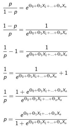
which can also be written as:
The equation:
is known as logit function and in the case of Logistic Regression gives us the probability, given the predictors, of an event being True.
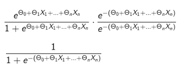
If, for sake of simplicity, we make for a moment:
![]()
we have:
 where t is the log of the odds
we can see that the above function is defined for any value of t. Moreover, when t = 0, P = 0.5
![]()
If we calculate the first derivative:

we see that it positive for any value of t.
And the second derivative:

we see that it is equal to zero when:
![]()
which is when t = 0. For negative values of t, the second derivative is positive (logit function is concave up), for positive values of t, the second derivative is negative(logit function is concave down). Therefore we can sketch our logit function (which represents the probability of an event being True):
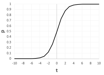
When the log of the odds is negative we have a probability of less than 50% of the event being True, when the log of the odds is positive we have a probability of more than 50% of the event being True.
The Cost Function
Our problem will be an optimization problem, which means finding the values of thetas
![]()
which minimize the Cost function, which for logistic regression, is the following:
![]()
where y is the observed outcome (True/False, or better 1,0) and p is the probability of the event being True given our parameters. Remember that:
![]()
When the observed outcome is 1 (True), (1-y) * ln(1-p) evaluates to 0, therefore only the part -y* ln(p) is considered and vice verse when the outcome is 0 (False).
If we quickly study the function ln(p) we see that:
![]()
![]()
and:


and because 0<=p<=1, over this interval the first derivative is always negative and the second derivative is always positive. Therefore we can sketch our function:
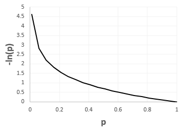
If we think about it, when the observed value is y = 1 (True), which is when the cost function is equal to -y * ln(p) = -ln(p), we want the ‘cost’ to increase as our prediction moves towards 0 (False, wrong prediction) and to decrease when our prediction moves toward 1 (True, correct prediction).
We can do the same kind of analysis when the observed value is y= 0 (False). Our cost function becomes -(1-y) * ln(1-p) = -ln(1-p). If we study this function, we get:
![]()
![]()


Therefore we can sketch this function:
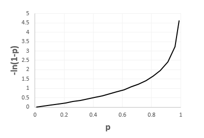
If we think about it, when the observed value is y = 0 (False), which is when the cost function is equal to -(1-y) * ln(1-p) = -ln(1-p), we want the ‘cost’ to increase as our prediction moves towards 1 (True, wrong prediction) and to decrease when our prediction moves toward 0 (False, correct prediction).
So our goal is to find the thetas which minimize this cost function. To do this, we will use the Truncated Newton Method within Scipy. But first, we need to calculate the gradient vector, the vector of partial derivatives for each of our thetas. I will show how to do this for Theta1, and luckly the process is the same for all the other thetas, so we’re in luck 🙂
I am showing below the whole procedure:
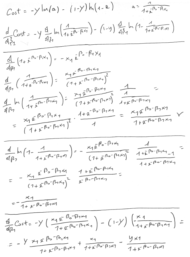
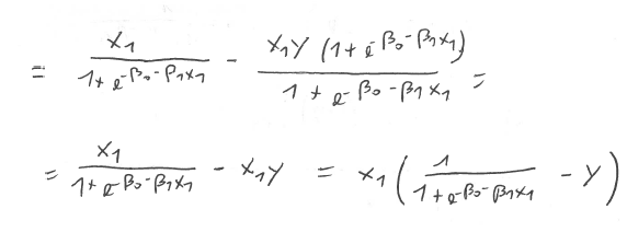
So, our gradient vector is:

Building a Logistic Regression Class in Python
In reality, because we will deal with many observation, the Cost function will be the sum for each observation of the Cost function shown above and divided by the number of observations, therefore it becomes:

and the gradient vector is like the one shown above, but with 1/m added:

remember that m is the number of observations, whereas n is the number of attributes. The gradient vector contains n+1 elements because X_0 is a column of 1’s which is multiplied against theta_0, the intercept. This makes matrix calculation easier.
The matrix of predictors is:

Our thetas vector:

and our observed outcomes:

The first method we will add will be called Sigmoid, which converts the log-odds vector into a probability vector:

This is very easy in Python using Numpy:
1 2 3 | def _sigmoid(self, data): # converts the log-odds to probabilities return 1 / (1 + np.exp(-data)) |
The second method will be used to calculate the cost function. Remember that the cost function is:
therefore, we first need to calculate the log-odds, then the probabilities and then the natural logarithm. In order to calculate the log-odds, which is:
![]()
we can perform a matrix multiplication between the predictors and the thetas:
then convert calculate the cost function:

the above will return a scalar value which will be divided by the number of the observations. Python code:
1 2 3 4 5 6 7 8 9 10 11 | def _predict(self, thetas, X): reshape_thetas = np.reshape(thetas, (-1,1)) # turn it into a N x 1 matrix log_odds = np.matmul(X, reshape_thetas) return self._sigmoid(log_odds) def _cost(self, thetas, X, Y): # returns the value of the cost function row_num, col_num = X.shape probabilities = self._predict(thetas, X) transpose_Y = np.reshape(Y, (1,-1)) # turn it into a 1 x M matrix from a M x 1 matrix return (np.matmul(-transpose_Y, np.log(probabilities)) - np.matmul(1-transpose_Y, np.log(1-probabilities))) / row_num |
The same things now needs to be done with the creation of the gradient vector, which will be a vector of the values of the partial derivatives.

letting the probability for i-th row equal to:
![]()
we can rewrite the gradient computation as:


which becomes:

1 2 3 4 5 6 7 8 9 10 11 | def _gradient(self, thetas, X, Y): ''' DESCRIPTION ------------------ returns the gradient vector of the cost function ''' row_num, col_num = X.shape probabilities = self._predict(thetas, X) differences = probabilities - Y gradient_vector = np.matmul(np.transpose(X), differences) / row_num return gradient_vector.flatten() |
How to calculate R^2 for Logistic Regression
There’re several ways of calculating r-squared for logistic regression. Here I will use the so-called McFadden Pseudo R-squared. The idea is very similar to r-squared of linear regression. In linear regression, r-squared as:

and it is the percentage of variation around the mean that goes away when you fit a linear regression model. It goes from 0 to 1. When fitting a line does not improve the variation around the mean, we get 0 and we’ve a very bad model. As the sum of squared errors goes down, R^2 goes up towards 1.
For logistic regression, we can first calculate the probability of an event being True without taking into account any of the predictors, therefore we only look at the observed outcomes and divide the number of Trues by the total number of observations, we will call it this probability o, and we will call the probabilities calculated by our model p.
Therefore, o is simply:
![]()
and p is:
and R-squared is:

you will notice the numerator is very similar to the cost function, which is also the case for linear regression.
Putting it all together, our class becomes:
1 2 3 4 5 6 7 8 9 10 11 12 13 14 15 16 17 18 19 20 21 22 23 24 25 26 27 28 29 30 31 32 33 34 35 36 37 38 39 40 41 42 43 44 45 46 47 48 49 50 51 52 53 54 55 56 57 58 59 60 61 62 | class LogisticRegression(object): def _predict(self, thetas, X): ' returns the probability of the event being True (1)' reshape_thetas = np.reshape(thetas, (-1,1)) # turn it into a N x 1 matrix log_odds = np.matmul(X, reshape_thetas) return self._sigmoid(log_odds) def _cost(self, thetas, X, Y): # returns the value of the cost function row_num, col_num = X.shape probabilities = self._predict(thetas, X) transpose_Y = np.reshape(Y, (1,-1)) # turn it into a 1 x M matrix from a M x 1 matrix ll_fit = self._LL_fit(thetas,X, Y) return -ll_fit / row_num def _LL_fit(self, thetas, X, Y): # returns the log likelihood of the data projected onto the best fitting line row_num, col_num = X.shape probabilities = self._predict(thetas, X) transpose_Y = np.reshape(Y, (1,-1)) # turn it into a 1 x M matrix from a M x 1 matrix return np.matmul(transpose_Y, np.log(probabilities)) + np.matmul(1-transpose_Y, np.log(1-probabilities)) def _sigmoid(self, data): # converts the log-odds to probabilities return 1 / (1 + np.exp(-data)) def _gradient(self, thetas, X, Y): ''' DESCRIPTION ------------------ returns the gradient vector of the cost function ''' row_num, col_num = X.shape probabilities = self._predict(thetas, X) differences = probabilities - Y gradient_vector = np.matmul(np.transpose(X), differences) / row_num return gradient_vector.flatten() def fit(self, X, Y): rows, cols = X.shape # add 1 column of 1's correspondent to the intercept #self.X = np.hstack((np.ones((rows,1), dtype=float), X)) self.X = X self.Y = Y # start with n thetas equal to 0 self.thetas = np.zeros((cols), dtype=float) # find the thetas which minize the cost function optimized = op.minimize(fun=self._cost, x0=self.thetas, args=(self.X, self.Y), method='TNC', jac=self._gradient) self.thetas=optimized.x def r_squared(self): ''' returns the McFadden's Pseudo R^2 ''' o = len(self.Y[self.Y == 1]) / len(self.Y) ll_intercept = np.sum(self.Y * np.log(o) + (1-self.Y) * np.log(1-o)) ll_fit = self._LL_fit(self.thetas, self.X, self.Y) return 1 - ll_fit / ll_intercept |
Now that we’ve our class, let’s use it to create some predictions, below is a simple project which uses the class we’ve just built to make breast cancer predictions:
Books I recommend to start your machine learning journey: