Excel People Connections Chart
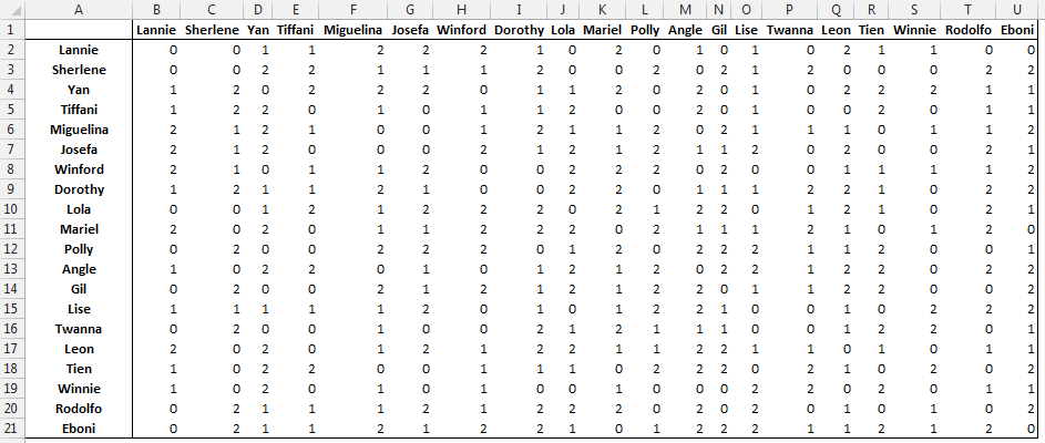
Suppose you have one table like the below which lists the relationship between two people: 0 No Relationship, 1 they just knows each other, 2 they are good friends. Excel People connections chart
I will show you the steps to build something like the below chart which connects all the people who are related (either 1 or 2) and which dynamically highlights the relationships of the person chosen:
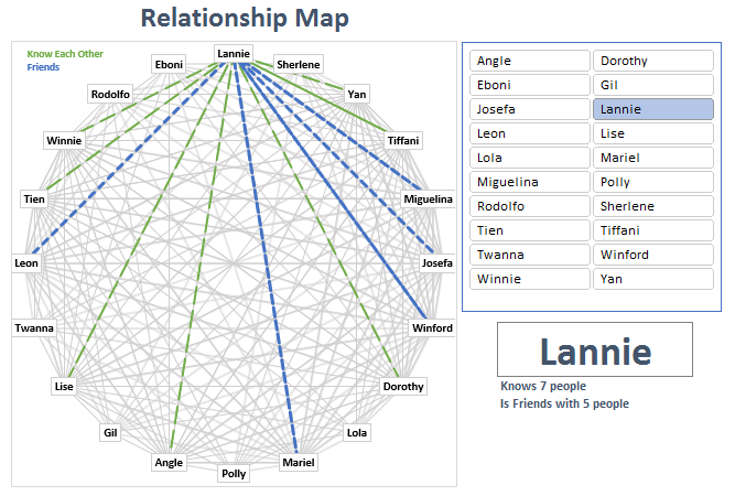
Excel People Connections Chart
Step 1 – Plot the names
To plot the names in circle we will need to calculate the coordinates of each point. For this we will need just a bit of trigonometry. There are 20 people, this means our circle needs to be divided into 20 parts of equal lengths. We know that a circle is of 360 degrees, this means each part is 360 / 20. So the first person needs to be at a degree of (1-1) * (360 / 20), the second person needs to be at (2-1)*(360/20) and so on. This is shown in column X on the tab People of the file whose link is at the beginning of the post. Once we know the degrees, we calculate the radians (column Y) and once we have the radians we calculate sine and cosine.
Select the data in column Z and AA and create a scatter plot chart with markers and no lines and remove all the gridlines, axis labels, set the axis min and max to -1 and 1 respectively. Then you can add the labels using the feature (Add values from Cells).
Step 2 – Build the lines for the relationships
The coordinates for the lines are on the tabs named Knows and Friends. The only difference between the two is the value in cell A1, where it is 1 for the tab Knows and 2 for the tab Friends. Each tab is divided into 20 sections (one per each person) of 4 columns each (recognizable by the borders). The formula in the first column returns a pattern of 3 values: first value is always the name of the person of that section, second value is the name of person, third is a blank cell. The second column returns the type of relationship (0, 1 or 2) and the third and fourth column return the coordinates of the person in the first column if the relationship (second column) matches the value in cell A1. Once you have these two tabs completed, it is easy to select columns 3 and 4 of each section (one section at a time) and add them to the chart as Scatter with lines without markers (I used a bit of VBA to add them all at once and formatted the Knows lines thinner and the Friends lines thicker).
Step 3 – Build the relationship lines for the highlighted name
The data for these lines is on the tab Highlight. The calculation is similar to the previous two tabs but in this case we want to retrieve the data only for the person chosen via the Slicers. Then I have formatted the Friend lines in strong blue and the Knows lines in green.
Additional Display
On the tab named Chart, you will find on the left the chart and on the right a sort of ‘Popularity Tables’ which you can sort in different ways to discover who are the most and least popular people:
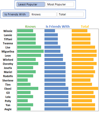
Excel Relationships Chart
This is a cool way of displaying people connections in a chart, I hope you will find it useful and you can build on it and make it even more insightful.
Hi,
how can I buy a copy of you file to test if it can display relationships between installed apps in an Odoo-database?
Hi Fredrik. Did you try the download link in the article?
Hi, this is fascinating. I would like to know if I can add more than 20 people? Is it hard for non expert user like me to do an adjustment?
HI there, is this based on graph theory? is there a way to represent this as a paths or hamiltonian?
hi there, i am stuck on step 2, on column B where it should return the relationship. in my case i have 21 people and i only want to know if they are connected or not so i basically won’t use the second tab. i can’t make this formula work 🙁 can you help me? what am i doing wrong? =CHOOSE(MOD(ROWS(A$4:A4)-1,3)+1,INDEX(relationships,MATCH(A5,people.row,0),MATCH(A4,people.row,0)),B3,””)
HUGE Thanks for publishing this article!!!