Ranking in Excel
You can use two different function for ranking in Excel: RANK.EQ and RANK.AVG. These two functions do essentially the same job but return different results for the items in your data set that tie. We will see how in the following examples.
Rank City Populations
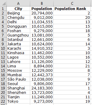
The first example has no ties in the data set. If you are sure that there are no ties then using either function will yield the same results.
Ranking in Excel
Place in C2 the following formula and drop down:
=RANK.EQ(B2,B$2:B$22,0)
The 0 in the formula indicates that you are sorting the values in descending order, to sort in ascending order use 1.
Results with ties
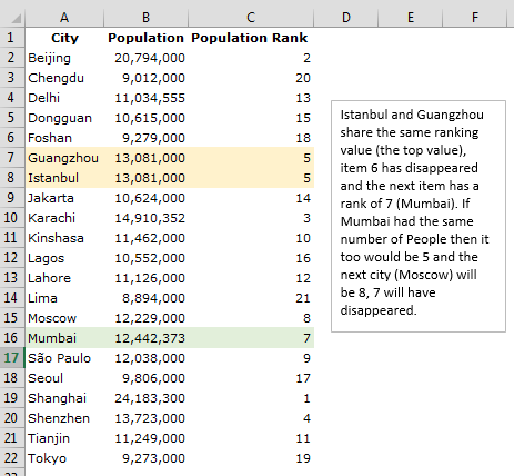
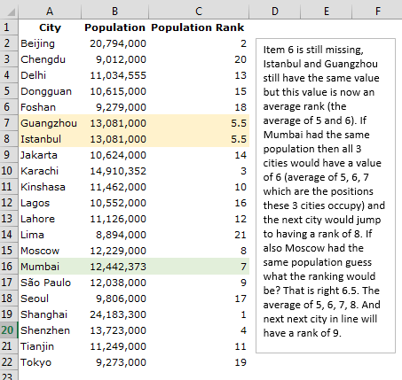
As I have mentioned earlier, when you have ties these functions will behave in a different way: RANK.EQ will return the same ranking value for the items that tie, whereas RANK.AVG will return the average rank for the same values. An example will explain this better.
Example with RANK.EQ
Ranking in Excel
Example with RANK.AVG
Ranking in Excel
Ranking with multiple conditions
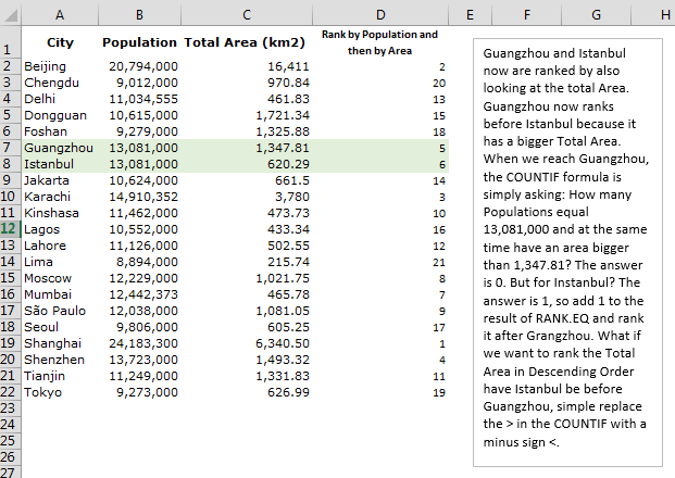
So far our examples included just one column by which we are performing the ranking. If you want to add extra conditions, that is to say rank by City Population and then rank the results that tie by the Total Area, we need to use a combination of RANK.EQ and COUNTIF.
The formula in D2 is:
=RANK.EQ(B2,B$2:B$22,0)+COUNTIFS(B$2:B$22,B2,C$2:C$22,”>”&C2)
Ranking in Excel
Ranking using only COUNTIF(S)
The above ranking can also be performed exclusively with COUNTIF(s).
=COUNTIFS(B$2:B$22,”>”&B2)+COUNTIFS(B$2:B$22,B2,C$2:C$22,”>”&C2)+1
On Beijing, the formula is saying: How many items are above 20,794,000? The answer is 1. Then it is saying how many items are equal to 20,794,000 and at the same time higher than 16,411 the answer is 0. So 1 + 0 = 1 and add 1 to this value so 2. Beijing is ranked number 2.
Advantages of using COUNTIF(S)
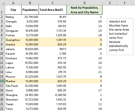
COUNTIF(s) brings a huge advantage when we need to rank items because it also works with text values whereas Rank.EQ and RANK.AVG don’t. Formula used in D2
COUNTIF(B$2:B$22,”>”&B2)+COUNTIFS(B$2:B$22,B2,$C$2:$C$22,”>”&C2)+
COUNTIFS($B$2:$B$22,B2,$C$2:$C$22,C2,$A$2:$A$22,”<“&A2)+1
Ranking in Excel
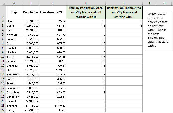
By using COUNTIF(s) you can also easily exclude some of the values from the Ranking. For instance, using the previous example, let us suppose you wish to exclude from the Ranking cities beginning with the letter D. The formula would become:
=IF(LEFT(A2,1)=”D”,””,COUNTIFS(B$2:B$22,”>”&B2,A$2:A$22,”
<>D*”)+COUNTIFS(B$2:B$22,B2,$C$2:$C$22,”>”&C2,A$2:A$22,”
<>D*”)+COUNTIFS($B$2:$B$22,B2,$C$2:$C$22,C2,$A$2:$A$22,”<“&A2,A$2:A$22,”<>D*”)+1)
Ranking in Excel
PERCENTRANK Function
Another way or ranking in Excel is using the PERCENTRANK function which ranks values as a percentage of your data set. PERCENTRANK will accept three arguments: the array or data set, the value to rank and the significance which is the number of decimals the function will return. If the value you want to rank is inside the data set the function is equivalent to doing: (RANK.EQ(ValueToRank,DataSet,1)-1)/(COUNT(DataSet)-1)
If the value you are going to rank is not in the data set then PERCENTRANK will perform an interpolation. It will sort the data set ascending, then it will find the value just before the one you are going to rank and the value just after.
The result will be: PERCENTRANK(Array,SmallerValue)+ (Mark * (PERCENTRANK(Array,HigherValue) – PERCENTRANK(Array,SmallerValue))
where Mark = (Value to Rank – Smaller Value) / (Higher Value – Smaller Value)
Post your comment if something is not clear or if you want to add new ways of ranking values!